- CT day 12, July 11, Tuesday
- Start: Collegiate West mile 21.4
- End: Collegiate West mile 43.5
- Miles walked: 22.1
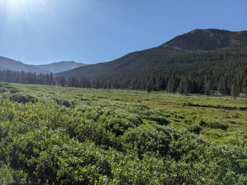
Taking a good while to descend off the mountain, the trail finally arrives at a trailhead and proceeds at the edge of a wetlands along Texas Creek.
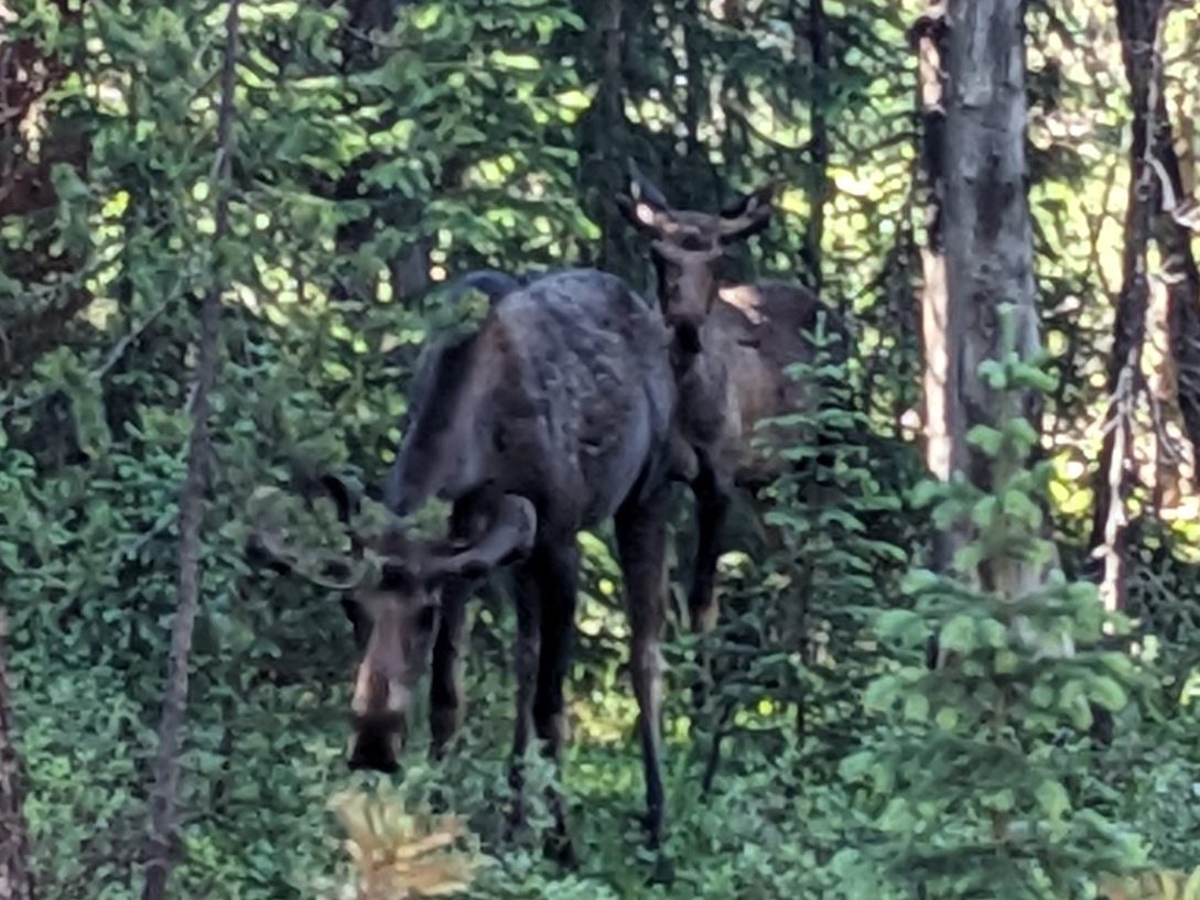
I hear a soft animal call and see a group of four moose grazing nearby– a bull, two cows, and a calf, their dark coats blending with forest shadow.