Sometimes I geek out in a long post about an arcane technical subject tangentially related to hiking. This is one of those. Reader beware.
Earbuds
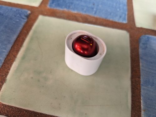
While doing long hikes I like to listen to audiobooks, and also podcasts on my cellphone. My bluetooth earbuds of choice are these tiny tiny ones, with good battery life and acceptable, though not exceptional, audio, that do not have a silicone ear canal gasket or attempt to block or cancel outside sounds. These are intended to be used in a single ear, so I can still hear nature sounds and be aware of my surroundings, essential for safe hiking.

One can pause/restart audio on this earbud with a single-press of the tiny button, but skipping forward requires a triple-click, instead of the more typical long-press or double-click. I can only guess these were designed for a market where advertisements were not thoroughly infesting podcasts, like we have here in North America. Doing triple-clicks on a tiny earbud button many dozens of times a day is just not practical.
Growth of Podcast Ads
According to Magellan AI‘s survey of podcasts, the average percentage of total ads in a podcast was 5.95% in Q2 2023, and jumped to 9.11% in Q2 2024. For some genres, like True Crime, the percentage is even worse: 17.23% in Q2 2024.
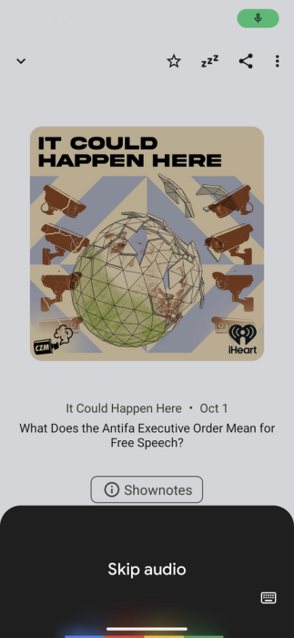
These figures sound low to me, so I noted ads in one episode of a typical podcast in my listening queue:
| Time | Content WLG 10/2/2025 |
| 00:00 | iHeart bumper |
| 00:04 | Camry ad in Spanish |
| 00:38 | Scottsdale ad |
| 01:05 | Thin nicotine ad |
| 01:30 | Granger ad |
| 02:06 | CoolZone bumper |
| 02:10 | podcast with music intro |
| 19:33 | Washable Sofas ad |
| 20:35 | Toyota ad in Spanish |
| 21:02 | Scottsdale ad |
| 21:35 | Granger ad |
| 22:07 | podcast |
| 31:12 | Washable Sofas ad |
| 32:15 | Toyota ad in Spanish |
| 32:48 | Scottsdale ad |
| 33:14 | Granger ad |
| 33:45 | podcast |
| 38:34 | podcast outro and credits |
| 39:10 | Toyota ad in Spanish |
| 39:40 | Scottsdale ad |
| 40:10 | Colgate ad |
| 41:00 | Amazon streaming ads |
| 41:30 | iHeart bumper |
| 41:34 | FIN |
Nineteen ads and bumpers in a 41:34 podcast total 9:29, or a 23% ad load! Several ads repeated multiple times, particularly annoying to listeners. None of the ads exhibited the humor or originality of a Superbowl-style ad, sadly. Hey companies, you are spending real money to get our attention, so why bore or annoy us?
I need an easy way to skip ads in podcasts while hiking.
Phone Hardware Buttons
As an alternative to the teeny tiny button on my earbud, I could pull out my phone, activate and unlock the phone screen, and tap the Skip-Forward button on my podcast player to get past ads, but that is not terribly practical to do often. Perhaps there is an app that uses a hardware button on the phone, like Volume Up, to skip forward?
There is! The one I use is Button Mapper, and I paid for the Pro version, which allows the app to function when the phone screen is off.
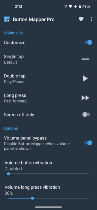
Particularly helpful is the option to give haptic feedback, with a vibration when the button is long-pressed.
Android made it hard for Button Mapper to work while the screen is off, unless you have a rooted device, but the developer figured out a way, using a work-around, using an adb (Android debugger) command, which is almost black magic to me.
Unfortunately, every time you reset the phone, you would have to repeat the adb command from an external computer. That is impractical on a long trail, in the event that you have to reset the phone to convince the cell function to start working again. However, the developer documents another way to get this functionality, using the Shizuku app. This is really and truly wizardry. I would, at this point, just give up and root my phone, or replace stock Android with GrapheneOS or LineageOS, but I use my phone to test a few apps I have developed, and need to know how the apps work with a phone that has normal permissions.
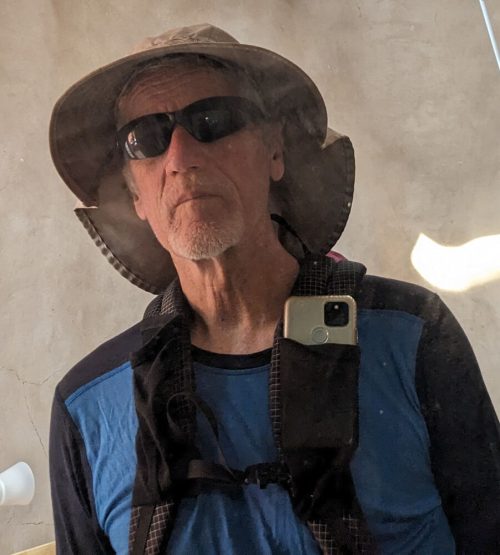
I normally carry my phone secured in a mesh pocket of my backpacking strap. With practice, I can long-press the phone volume button through the mesh without taking the phone out, and on a long hike the process becomes automatic.
By using long-presses on either the Volume-Up button and the Volume-Down button to perform the same Skip-Forward function, I do not have to be very precise on hand placement on the button.
Tappy Tap-Tap
A few years ago, I tried to develop an app that detects a pattern of taps on the back of the phone, using the built-in accelerometer sensor in the device, and performs some action. I never got it to work reliably, and never released the app. I was trying to filter out all the vibration and noisy signal programmatically, using simple DSP filters, and I probably should have used machine learning instead, but I did not have that skill.
Great minds think alike. Google now has a feature on Pixel Phones called Quick Tap, which recognizes a double-tap or triple-tap gesture on the back of the phone, and performs some actions as a result.
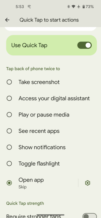
Google does not offer “Audio Skip Forward” as an option, but it does offer “Open app”. So I wrote an app that causes the application that is currently playing audio to skip forward. Normally apps are not allowed to broadcast KeyEvents to other applications, without special very high permissions, but there is an exception for broadcasting media keycodes like “skip forward” KeyEvent.KEYCODE_MEDIA_SKIP_FORWARD or “fast forward” KeyEvent.KEYCODE_MEDIA_FAST_FORWARD. My custom app code is very small, with the important method below:
public class MainActivity extends AppCompatActivity {

    @Override
    protected void onCreate(Bundle savedInstanceState) {
        super.onCreate(savedInstanceState);

        AudioManager am = (AudioManager) getSystemService(Context.AUDIO_SERVICE);

        am.dispatchMediaKeyEvent(new KeyEvent(KeyEvent.ACTION_DOWN, KeyEvent.KEYCODE_MEDIA_SKIP_FORWARD));
        am.dispatchMediaKeyEvent(new KeyEvent(KeyEvent.ACTION_UP, KeyEvent.KEYCODE_MEDIA_SKIP_FORWARD));

        am.dispatchMediaKeyEvent(new KeyEvent(KeyEvent.ACTION_DOWN, KeyEvent.KEYCODE_MEDIA_FAST_FORWARD));
        am.dispatchMediaKeyEvent(new KeyEvent(KeyEvent.ACTION_UP, KeyEvent.KEYCODE_MEDIA_FAST_FORWARD));

        finishAndRemoveTask();
    }
}
(My app Skip does not act like typical Android apps, because it does not have a screen display or any controls or settings, and only does one thing upon startup and immediately exits, more like a Unix-style shell program. Skip is so different from other Android apps that it would probably not be well received on the Google Play Store.)
My app works with Quick Tap! But unfortunately it does not function with the phone screen off. I suspect the reason is that Google is continually restricting what apps are able to do for each new Android version, in the name of security, and at some point they started preventing apps from launching other apps when the screen is off, unless the first app has a special permission. I could be wrong, but it appears that Quick Tap does not appear to have this permission on the Pixel 5.
However, some developer created an open source app, called Tap Tap, which adapted Google’s code for Quick Tap, and expands its capabilities. It adds several built-in media control commands, but not exactly what I need for my podcast player to skip ads . It took a lot of doing, but I can configure Tap Tap to run in Accessibility Mode, which allows it to launch an app when the screen is off! So now, on my next hike, I am able to skip commercials with a double-tap of the back of my phone, while it is located in my pants pocket or in my backpack strap mesh pocket.
I do notice that Android sometimes kills the Tap Tap service, and I have to start it again.
Tap Tap seems to draw more power, which could be an issue on long hikes, where cell phone power consumption is a limiting factor to how often I can listen to audio each day.
Hands Free
Often I want to control phone audio when both hands are occupied, holding trekking poles or encased in gloves. Can I use speech commands to skip forward? I do not particularly want to enable “Hey Google” on my phone, because Google listening to audio and keeping recordings indefinitely creeps me out, but let’s try it anyway for skipping audio.
After enabling Google Assistant on my phone, I noticed the app is very good at recognizing my voice for wake-words and following commands. However, there is a timing gap before receiving the beep acknowledging the wake-word and ready to receive a command. The whole cycle of saying the wake-word, waiting for the beep, saying the command “skip audio” or “launch Skip”, and waiting for the command to be interpreted is a few seconds, not ideal when you might have to skip several minutes of a podcast commercial break. Assistant is supposed to have a “Quick phases” feature, where you can skip the “Hey Google” wake-word for certain frequently-used commands, but that feature works with Pixel 6 or later, and I have a Pixel 5.
What’s worse, Google Assistant will not work in Airplane mode, at least not at the time of this writing, and on my Pixel 5. It interprets the “Hey Google” wake-word just fine, but will not carry out a command. Something odd is going on here. When in Airplane mode Google Assistant recognizes my speech command just fine:
But apparently Assistant does not know how to interpret the command: It insists on trying to connect to Google:
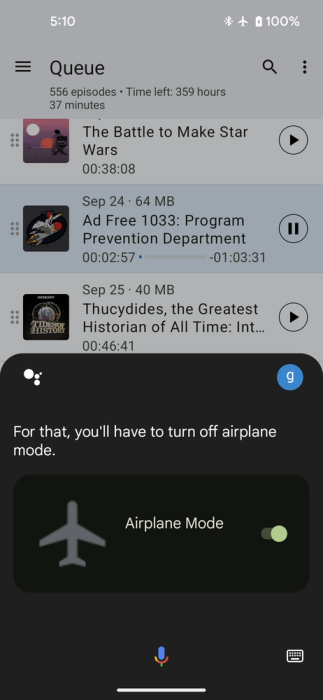
For this reason, Google Assistant (at the time of this writing, and with my model of phone) is useless for hands-free control on long hiking trips, when we expect to be out of communication range most of the time.
Interestingly, I found an article from 2015 that stated that the earlier version of Google voice commands could perform limited commands off-line, including launching an app.
Dicio assistant is an open-source off-line hands-free assistant.
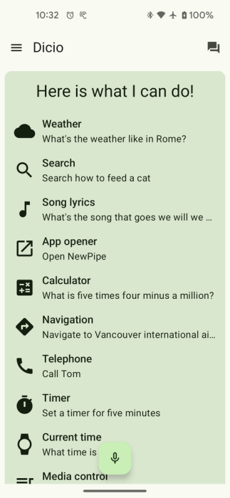
It works completely off-line, and thus preserves your privacy.
Dicio assistant is an ambitious project, but there are issues:
- For me, voice recognition did not work as well as Google Assistant.
- I still run into the problem of the total time of saying the wake-word, getting the recognition beep, and saying the command taking too long.
- I could not get Dicio to launch another app. I suspect this is due to what I call Android Upgrade Blight: Google keeps changing APIs and restricting permissions of apps in the name of security for each Android release, and it is hard for developers to keep up with changes. Starting in Android 14, Google added an explicit opt-in permission requirement in order to allow launching of apps.
- In any event, using Dicio to launch my Skip app would not work, because my app sends the fast-forward request to the app that currently has audio focus, which in this case would be Dicio telling me it just launched my app, and not my podcast player.
- Dicio is extensible and does allow people to add other skills. While their current built-in media control skills do not include “skip-forward”, this skill could theoretically be added, but would take quite a bit of research on my part to understand their skill format.
- I still haven’t tested the power requirements of running Dicio or another assistant in the background
- It is not clear how a voice assistant would perform in the field on days when there could be quite a bit of wind noise.
Future Hacks
An open-source wake-word library exists, and another is targeted specifically for Android, so what if I bolt that library onto to my Skip app, so that a simple “Hey Skip” voice command issues a command to skip audio by one minute, without any “Hey Google” or “Hey Dicio” preamble? Perhaps you would like to experiment with this idea, or alternatively subscribe to this blog to be notified of my future experiments.
Have I missed some alternative for skipping ads? Do you have suggestions or questions? Leave a comment on this post..
Related Posts: