Trails and Graph Theory 4 : Import Maps

We will use the OSMnx library to import trails from OpenStreetMap to our graph. Installing the library typically requires more than the Python pip utility– use conda, and follow on-line guides– pretty much black magic to me. The folium library is used to display our maps with graphs.

import osmnx as ox
import networkx as nx
import folium

ox.settings.log_console=True
ox.settings.use_cache=True

Let us import a trail network.

# location where you want to find your route
place = 'Gila National Forest, New Mexico, United States'

We will create a custom filter to only import trails. If we use the default network_type=’walk’ we also get dirt forest roads. Also, make retain_all=True instead of the default, or we will discard disconnected subgraphs, such as the entire Aldo Leopold Wilderness!

cf = '["highway"~"path|footway"]'

graph = ox.graph_from_place(place,
   simplify=True,retain_all=True,custom_filter=cf)

len = ox.stats.edge_length_total(graph) #in meters
len = len * 0.0006213712
print(f'total length {len:.2f} miles') 

     total length 2839.50 miles

(The total length of trails might be inflated by a factor of 2, because graph is a multidigraph, so edges are doubled.)

For practice we will define a couple of points and find a shortest distance on trail.

#intersection Spring Canyon Trail #247 and Gila River Trail #724
start_latlng = (33.04876, -108.30680)

#intersection Trail #187 and Turkey Creek Trail #155
end_latlng = (33.26496, -108.45945)

# find shortest path based on distance or time
optimizer = 'length'        # 'length','time'

# find the nearest node to the start location
orig_node = ox.distance.nearest_nodes(graph, start_latlng[1],
                                      start_latlng[0])
# find the nearest node to the end location
dest_node = ox.distance.nearest_nodes(graph, end_latlng[1],
                                      end_latlng[0])

#  find the shortest path
shortest_route = nx.shortest_path(graph,
                                  orig_node,
                                  dest_node,
                                  weight=optimizer)

print(shortest_route) 

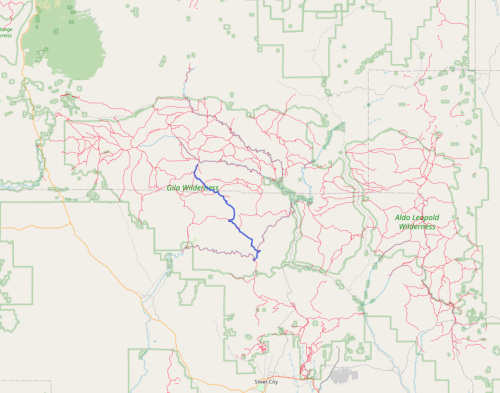
 [2506756220, 142157900, 9775068479, 9775034297, 2509002117, 2509002850, 2509002755, 2509004058, 2509005091, 2509005336, 2509005784]

Using folium, we can create a trail map, and highlight the shortest route calculated above.

m = ox.plot_route_folium(graph, shortest_route,tiles='openstreetmap')

graph_options = {
    "weight": 1,
    "color": '#ff0033',
    "opacity": 0.3,
    "width": 5,
}
ox.folium.plot_graph_folium(graph,m,**graph_options)

# include the option to switch map layers
folium.TileLayer('openstreetmap').add_to(m)
folium.TileLayer('Stamen Terrain').add_to(m)
folium.TileLayer(
  tiles='https://{s}.tile-cyclosm.openstreetmap.fr/cyclosm/{z}/{x}/{y}.png',
  name='cyclosm',
  attr='CyclOSM',
  ).add_to(m)
folium.LayerControl().add_to(m)

m.save("play_map2.html")
m.show_in_browser()

Now, the trail map may need some fixes, like adding/deleting trails, and including a few dirt roads to connect the eastern trails with the rest of the network, but think how far we have come…

We shall save the graph to disk, to be used for later analysis.

ox.io.save_graph_geopackage(graph, filepath='gila_trails.gpkg')

Related Posts:

• Trails and Graph Theory: The Series