After adding a few short roads to fill in gaps to a trail network, my algorithm (for finding the longest continuous loop without repeating any trail section) hit a brick wall, and stopped giving improving results. It seems my code has some edge cases that were not being handled correctly with the new expanded network, and sleuthing is required.
I will go through fixing edge cases in the next post, but here we show some ways to visualize the trail graph, which will aid in debugging.
Color Nodes and Edges
Important in our algorithm is whether nodes have three edges or four, and we can color nodes and edges to help see what is going on. Here we use the cmap argument in the map drawing function explore.
geopandas.GeoDataFrame.explore(column,cmap,folium.Map, tiles, ... , **kwargs)
The cmap takes some attribute and translates it into a color. The particular color is calculated using the maximum/minimum range for the attribute, and calculates a color within the cmap spectrum. Several pre-built cmap spectrums are already defined in the matplotlib library. I do not particularly care what colors are chosen, as long as they are visually distinct. Here are a couple of cmaps I have used.


Let us name the attribute we add to nodes and edges ‘color‘, and calculate colors for nodes, like so:
    for node, dat in Q.nodes(data=True):
        d = Q.degree(node)
        dat['color'] = d
The way the cmap is used in the explore function is like this:
m = edges.explore(column='color', cmap = 'tab10', legend=False, tiles="openstreetmap")
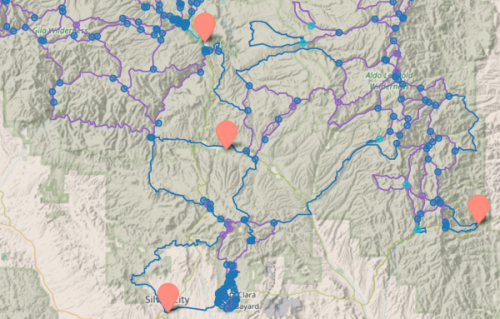
And when we draw a trail map, nodes and edges appear to help us diagnose trail connections.
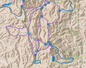
For this map, nodes with odd number of edges are in blue, and nodes with 4 edges are in turquoise. Trails are purple, and road sections are turquoise.
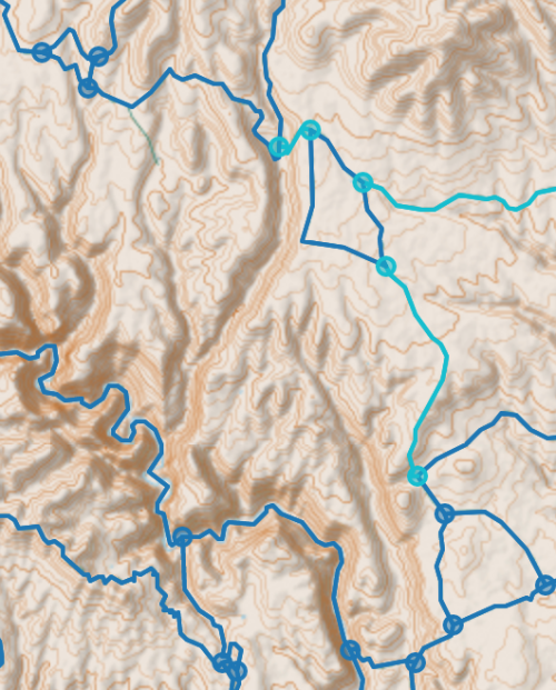
We can add extra colorize functions to explore other properties of the graph. A bridge on a graph is an edge that, if cut, divides the graph into separate subgraphs. Bridges are a measure of the connectivity of an edge. When we start eliminating edges so that all nodes are even, we probably do not want to break up the graph very much, so in the future we may weight these edges to minimize the chance of deleting them. Find bridges in a graph with the Networkx function:
nx.bridges(T)
And we write a function colorize_edge_list to highlight these edges:
bridge_list = list(nx.bridges(T))
print('length of bridges:', len(bridge_list))
T = colorize_edge_list(T, bridge_list)
draw(T,'bridges on simplified graph', show_nodes=True)
During debugging, one can imagine writing several special-purpose colorize_xx() functions, for highlighting matched nodes, displaying unmatched nodes, showing all 4nodes that are connected directly to another 4node, and so forth.
While working with our draw() function, we might as well add or fix a few other features.
Tool Tip (Hover Text)
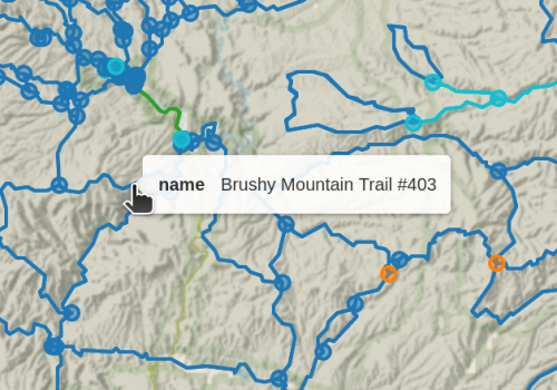
Previously when hovering over edges on our map, all attributes were displayed, which is rather ugly.
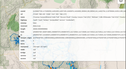
But the explore function has argument that selects which attribute, or column, do display as a tool tip, and ‘name’ is a good option for OSMnx plots:
m = edges.explore(column='color', cmap='tab10', legend=False, tiles="openstreetmap", tooltip='name')
Town Markers
We had previously used Markers to display features we were debugging, such as small gaps in our trail network. Now we choose to use markers to display potential trail resupply towns. The display code is already written, located in the draw() function several blog posts ago, so the only thing left is to add the array of town GPS coordinates.
town_markers = [(34.29963, -108.13268, 'Pie Town'),
         (33.19593, -108.20834, 'Gila Hot Springs'),
         (32.77981, -108.27533, 'Silver City'),
         (33.37939, -108.90369, 'Alma/Glenwood'),
         (33.03022, -108.16864, 'Lake Roberts'),
         (32.91685, -107.70593, 'Kingston')]
Three Dimensions
Looking towards the far future, assuming my tools are debugged to find a good long distance hiking route, it would be really great if we could view our trail in 3D, for planning a hike. OpenStreetMap.org does not currently have a 3-D display option, but height is included in OSM data. A few open-source projects do display OSM in 3D. OSM Buildings is one effort, but seems oriented towards city buildings.

Another project is Streets.gl, which looks better for what we want.
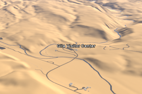
As far as I can discover, the website only displays roads, and not trails, but it is open source, so this might be a great project for any of you trail geeks.
Source code for coloring will be included in the next post, which should come out soon.