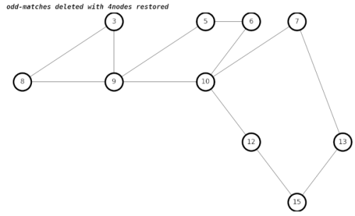
After adding in a few short sections of road to my trail graph, which should make it more connected and allow a longer route, I was noticing poor performance. The longest route was not getting particularly long, and typically a matching would not be complete– there would be leftover odd nodes, and also unmatched nodes, so eliminating matched edges would not result in a Eulerian graph.
length of min_weight_matching =  163
is perfect matching?  False
node  2510903794  not in matching
node  2834068719  not in matching
Let us remind ourselves of the algorithm:
- Simplify graph (remove all 2nodes)
- Remove ends (remove all 1nodes)
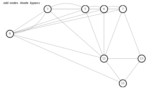
- Make odd-node graph by deleting 4nodes
- For all 4nodes in original graph, add temporary bypass edges to odd-node graph, which should still be odd-node. If it is not all odd-node, you did something wrong.
- Match odd nodes in pairs, using a matching algorithm
- Delete edge between matched pairs of nodes
- Replace any temporary bypass edges that still exist with the original edges
- Resulting graph should be all even nodes. If not you did something wrong!!!
- Graph is an Euler graph, which means you can find a continuous loop that includes all remaining edges.
My previous code is not entirely correct. Here are some situations that are (or may be) breaking this procedure:
Parallel Edges
In NetworkX a simple Graph object allows only one edge between any two nodes, but we are using a Multigraph, which can allow more than one edge between two nodes. The parallel edges are identified with their own key value, which is an integer in the case of the OSMnx library. Instead of iterating through edges as with a simple Graph:
for u,v in Q.edges():
we include the key in our iteration.
for u,v,k in Q.edges(keys=True):
My early code was fairly sloppy about this, and often forgot about parallel edges, so several functions needed to be updated. Also, code has been added to count the number of parallel edges in our report() function, which increases as part of the simplification function.
84539 nodes in largest subgraph
84730 edges in largest subgraph
total length 1573.54 miles in largest subgraph
number of odd intersections in largest subgraph : 606
number of even intersections in largest subgraph : 83933
number of 2-way intersections in largest subgraph : 83902
number of 4-way intersections in largest subgraph : 31
number of trailhead/terminus in largest subgraph : 145
number of parallel edges in largest subgraph : 0
number of 4-way adjacent pairs in largest subgraph : 1
354 nodes simplified graph
554 edges simplified graph
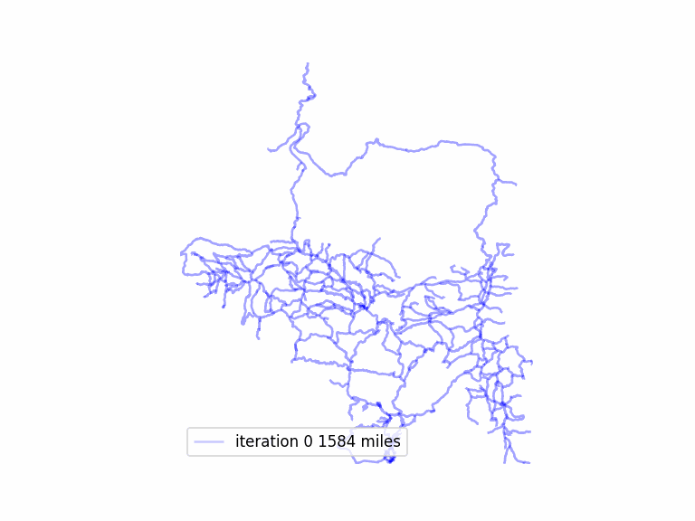
total length 1285.20 miles simplified graph
number of odd intersections simplified graph : 328
number of even intersections simplified graph : 26
number of 2-way intersections simplified graph : 0
number of 4-way intersections simplified graph : 26
number of trailhead/terminus simplified graph : 0
number of parallel edges simplified graph : 67
number of 4-way adjacent pairs simplified graph : 11
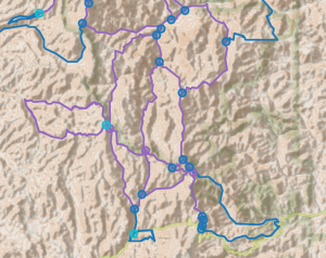
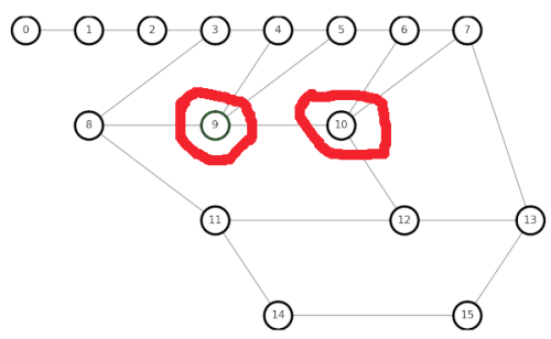
Adjacent 4nodes
My original code for making temporary bypasses is not entirely correct. It does not handle the case of a 4node connecting to a 4node neighbor. How many of those situations exist? From the above report:
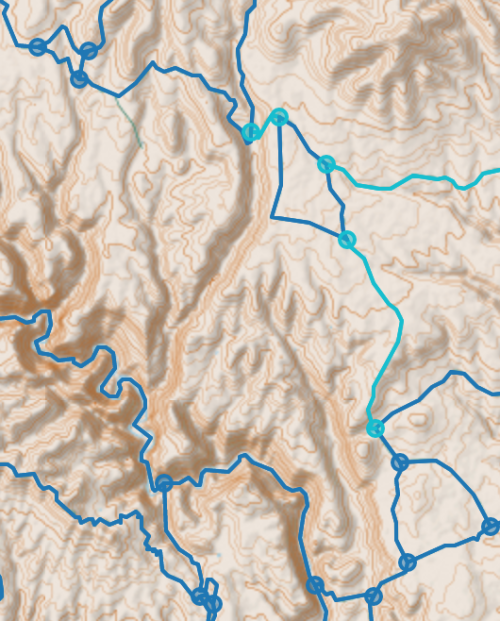
number of 4-way adjacent pairs simplified graph : 11I could not patch the existing code to handle 4node neighbors, even after attempting recursion, and had to start from scratch 2 or 3 times to get something that partly works. And in the image below there are 3 adjacent 4nodes connected in a chain, which my code still does not deal with well.
To debug my code, it is best to go back to simple small graphs to use for testing, as we did in Chapter 6. Let us create a graph with two adjacent 4nodes:
My earlier algorithm gives incorrect results when trying to restore 4nodes, which is not an Euler loop.

After a lengthy amount of hair-pulling during debugging, my new algorithm gives the correct results.
The way we get the correct result in graphs with adjacent 4nodes is to create temporary edges between each of the neighbors of both 4nodes, which becomes something of a hairball.
I am not entirely convinced that my code handles all cases of adjacent 4nodes correctly. Errors are lurking. The related Chinese Postman problem does not have these issues, because you are adding edges, not deleting edges. Deleting edges often breaks things.
4node Neighbors with Parallel Edges
Playing around with my small graph, I discovered another configuration that broke my algorithm. Two 4node neighbors that each share two edges between them seems to be a problem.
One solution is to delete one of the parallel edges, converting the neighboring 4nodes into neighboring 3nodes, which is easy for the algorithm. Somehow, I suspect that is not the optimal solution, but it is easy to code, so I will use it for now, until I see a problem with performance.
Later, I found that a 3node connected to a 4node with parallel edges also has this same problem, so I fixed it in the same inelegant way. Sigh.
Other Problem Topologies
Along with 4node neighbhors and 4node covalent neighbors, are there other topologies that might cause a problem with my algorithm? One possible way to test is to generate random planar graphs of about 15 nodes, iterating and searching for anything that breaks my algorithm. Perhaps later… something to add to the To-Do List.
Self Loops
Multigraphs also allow self-loops. I added code to count how many exist.
def check_self_loops(Q,txt=''):
    self_loops = 0
    self_loop_distance = 0
    max_self_loop_distance = 0
    for u,v,k,dic in Q.edges(keys=True,data=True):
        if u==v:
            d = dic['length']
            self_loops += 1
            self_loop_distance += d
            if d>max_self_loop_distance:
                max_self_loop_distance = d
    print('number of self-loops ' + txt + ' : ', self_loops )
    print(f'total self-loop distance {self_loop_distance*0.0006213712:.2f} miles ', txt)
    print(f'maximum self-loop distance {max_self_loop_distance*0.0006213712:.2f} miles ', txt)
    print('')
Here are the results:
number of self-loops simplified graph :  18
total self-loop distance 86.05 miles  simplified graph
maximum self-loop distance 16.78 miles  simplified graph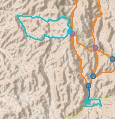
Compared to the graph mileage (1285.20 miles), the total mileage of self-loops is small. My code has trouble dealing with self-loops, especially calculating the number of edges on a node, so it is easiest to delete self-loops, and add them in later if we need to.
Difficult Nodes !!
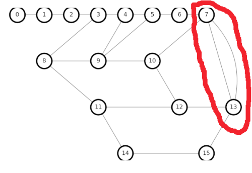
A small number of 3nodes tend to be difficult to match with other 3nodes using the built-in matching algorithms in the NetworkX library, such as min_weight_matching().
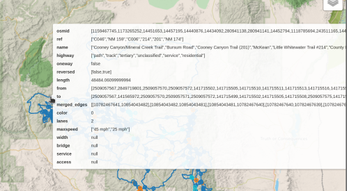
Here are some nodes that are not matching, through several iterations:
length of max_weight_matching =  163
is perfect matching?  False
node  2509005592  not in matching
node  2834068719  not in matching

length of min_weight_matching =  163
is perfect matching?  False
node  2510903794  not in matching
node  2834068719  not in matching

length of no-weight min_weight_matching =  163
is no-weight matching perfect?  False
node  2509003421  not in matching
node  2834068719  not in matching

node  6226321975  not in matching
node  2834068719  not in matching

node  2510903794  not in matching
node  2834068719  not in matching

node  2510903794  not in matching
node  2834068719  not in matching

node  2510903794  not in matching
node  2834068719  not in matching

node  2510903794  not in matching
node  2834068719  not in matching
To do a fully optimized matching, we should create a complete graph, where all nodes are connected to all other nodes using temporary edges with the trail distances between any two nodes on the graph. I am taking the short-cut of only calculating the distances between nearby nodes, and only adding temporary edges to skip over 4nodes. This may leave a few nodes in isolation, that almost never get matched. On earlier simulations these nodes might get eliminated when a subgraph got disconnected, so we could still find a perfect matching. And many subgraphs got disconnected. But now we have added a few roads to make a more connected graph, which gives us the advantage of finding a longer route, but increases the chance that we never find a perfect matching, which is necessary to find an Euler Loop. Additionally, at least one of the short roads added, to connect the Aldo to the rest of the Gila, tended to be one of those hard-to-match nodes.
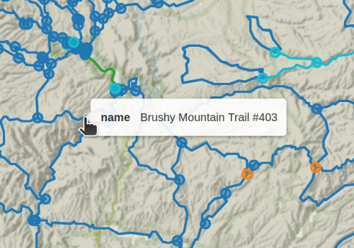
How do you find the location of a node with its node number (aka node id). I wrote code to colorize, but in general you can edit this URL and substitute the node you are searching for, and it will display on a map.
https://www.openstreetmap.org/node/2834068719(Do not try to put the node id in the search box for OpenStreepMap– it just doesn’t work for now.)
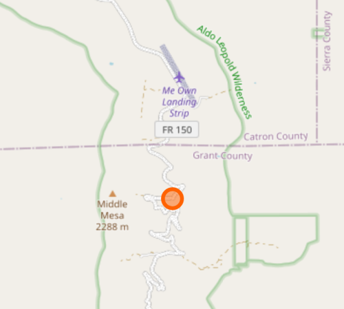
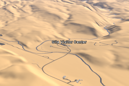
I really not want to eliminate this node, or any of the edges connecting it, since it bridges the Aldo to the Gila. Looking at my input map, I was actually missing a few good connections around “Me Own Admin Area” (which I am familiar with because the Grand Enchantment Trail passes through).
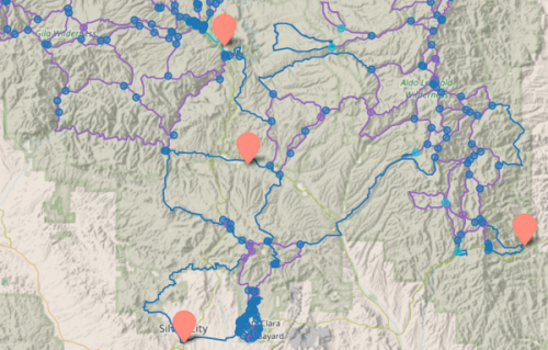
Adding a few extra short roads across the gap between the Aldo and Gila solved the problem, and missing trails re-appeared. I do not know if the previous graph had a data integrity problem, or a 3node was really isolated from potential matches, but anyway the problem disappeared, so on to the next adventure.
After all these fixes, I am still getting a high percentage of non-Euler graphs after matching. After many weeks of debugging, I needed a temporary fix to proceed.
A FINAL HACK…
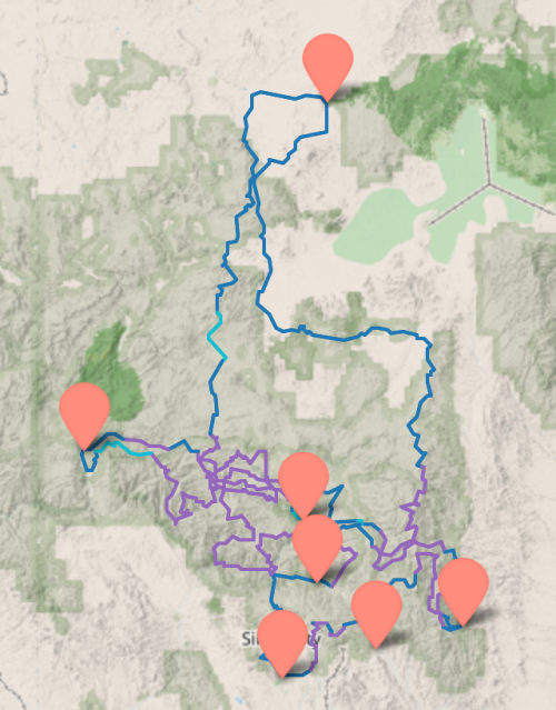
Eventually I realized that, with a recently upgraded computer, I could get around the problem of a high proportion of non-Euler graph attempted solutions: Each iteration only takes seconds to compute, so if I need to run 10,000 iterations to get 500 Euler graph solution candidates, that still did not take too long, and I could easily find loop trails more than 700 miles long, plenty long for a good hike. We may be stepping back from the original goal of finding the longest continuous non-repeating loop in the Gila, to finding one long enough. We may be missing better solutions with our buggy code, but those improvements can be made at a later time.
Inelegant and buggy source code may be downloaded here.