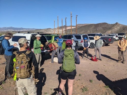
Ten volunteers from Socorro Trails joined a group from Rocky Mountain Youth Corps to finish the far loop of the Landavaso Trail just outside of Magdalena.
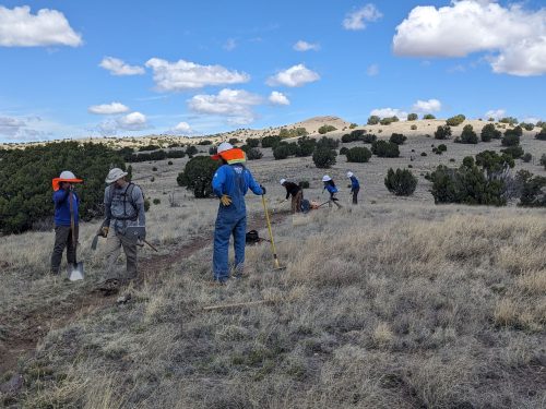

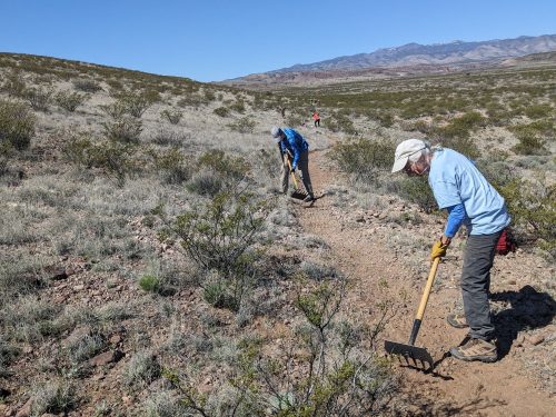
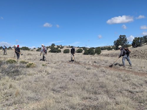
The Corps had already improved the far loop by the time we arrived, so we spent the entire day adding finishing touches, with emphasis on removing berm.
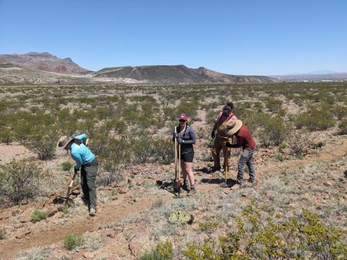
The trail appears to already be frequently used by local hikers, doggies, and bikes. If the highway department puts up a trail sign at the turn-off, usage will be even better.
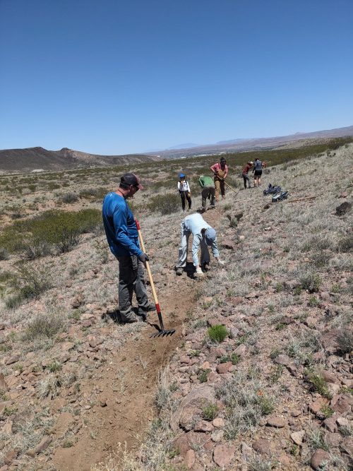
Grasses will try to grow a living berm along the trail each year, so we will be back.