- CDT NM 2025 Day 1, April 7
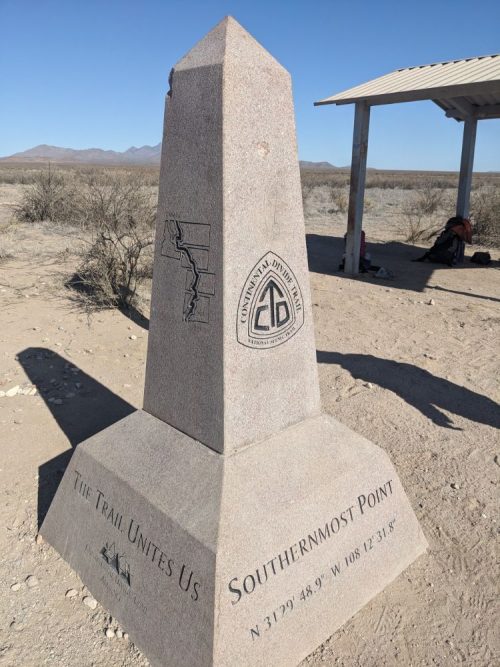
- Start Crazy Cook mile 0
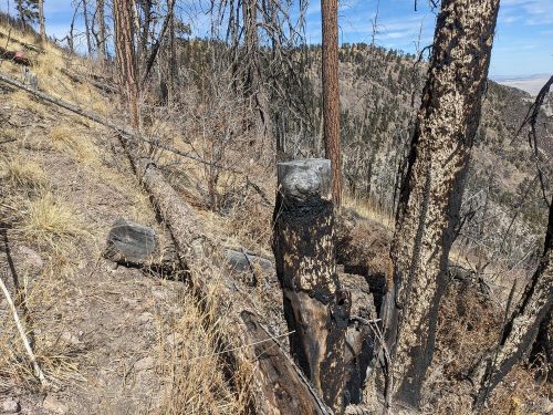
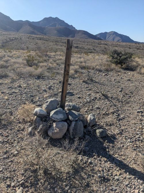
- End post and cairns mile 20.5
- Miles walked: 20.5
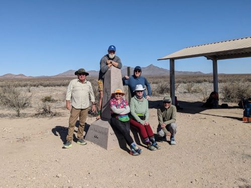
The Greyhound bus arrives in Lordsburg at 5:45AM, and the CDTC Shuttle departs at 6:30AM to the beginning of the CDT at the Mexico border, at Crazy Cook National Monument, arriving around 9AM.
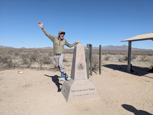
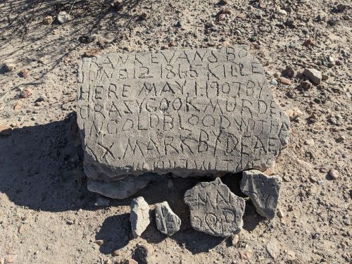
The monument gets its name from a murder at a cowboy camp in 1865, marked by a nearby crude stone marker.
The hikers starting off with me are Pancho, Mud Duck, Pikachu, Jess, and Tenderfoot.
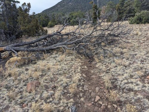
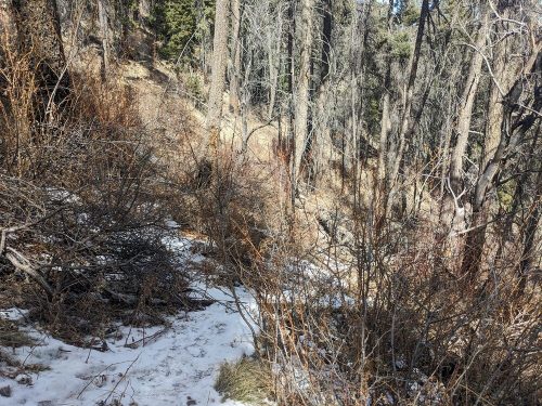
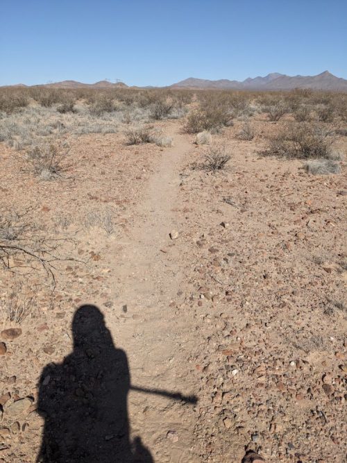
We start off walking among creosote bush on well-defined tread.
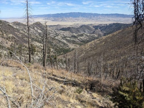
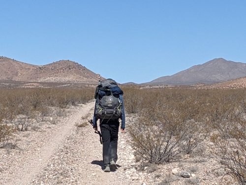
Soon the trail heads toward a gap in the hills. Tenderfoot and I pass each other several times during the day.
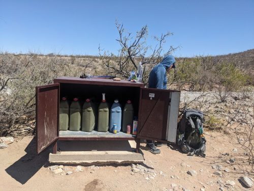
The first water cache is near mile 14, in a bear box.
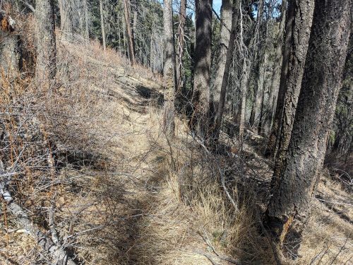
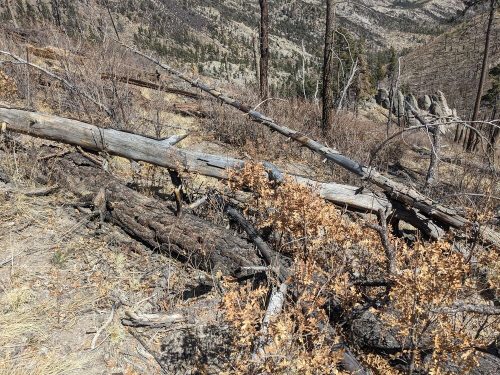
The trail here splits for a few miles, with one option continuing in a dry rocky creek bed, and another climbing up, marked with post-and-cairns. Tenderfoot and I choose the high route.
The next water cache box is near mile 44 (though there might be other water opportunities). My goal is to put in more miles today, to make it easier tomorrow.
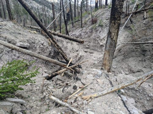
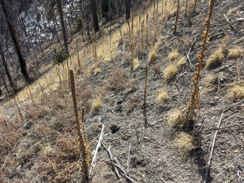
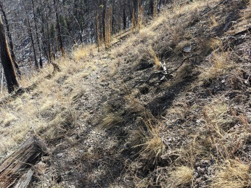
Sometimes it is hard to spot the next post marking the trail, and the tread is light and hard to follow. The route frequently goes down and up arroyos. I start to slow down, low on energy, and Tenderfoot is far ahead. I pause for a siesta, fall asleep for a few minutes, and eat first dinner. Continuing on, refreshed, I stop at dusk just after spotting Tenderfoot’s tent.